Visualization & Landscape Analysis

Visualization is an essential tool in optimization and system solving. It translates abstract mathematical landscapes—such as multimodal objective spaces with multiple local/global optima or non-linear equation systems with multiple roots—into intuitive visual representations.

pysne provides visualization tools built directly on top of matplotlib. You can run these tools as ready-to-use Command Line Interface (CLI) scripts or import their visualization functions directly into your own Python scripts via pysne.visualization.

---

Overview of Visualization Tools

Visualization Mode	Target Problem	Dimensionality	Description
SNE Equation Contours	SNEProblem	1D & 2D	Plots zero-level equation contours (\(f_i(\mathbf{x}) = 0\)) and overlays solver-discovered roots at contour intersections.
SNE Fitness Scatter	SNEProblem	3D	3D scatter plot thresholded at top fitness regions with 3D root markers.
Multimodal Surface & Heatmap	MultimodalProblem	2D	Side-by-side 3D Surface landscape and 2D Contour Heatmap with overlaid maxima and minima.
Multimodal 3D & Cross-Sections	MultimodalProblem	3D	3D thresholded scatter plot accompanied by 2D cross-sectional slice heatmaps.

---

Quick Start Tutorial (CLI Usage)

pysne visualizers act as convenient wrappers around matplotlib. You can execute them directly from your terminal.

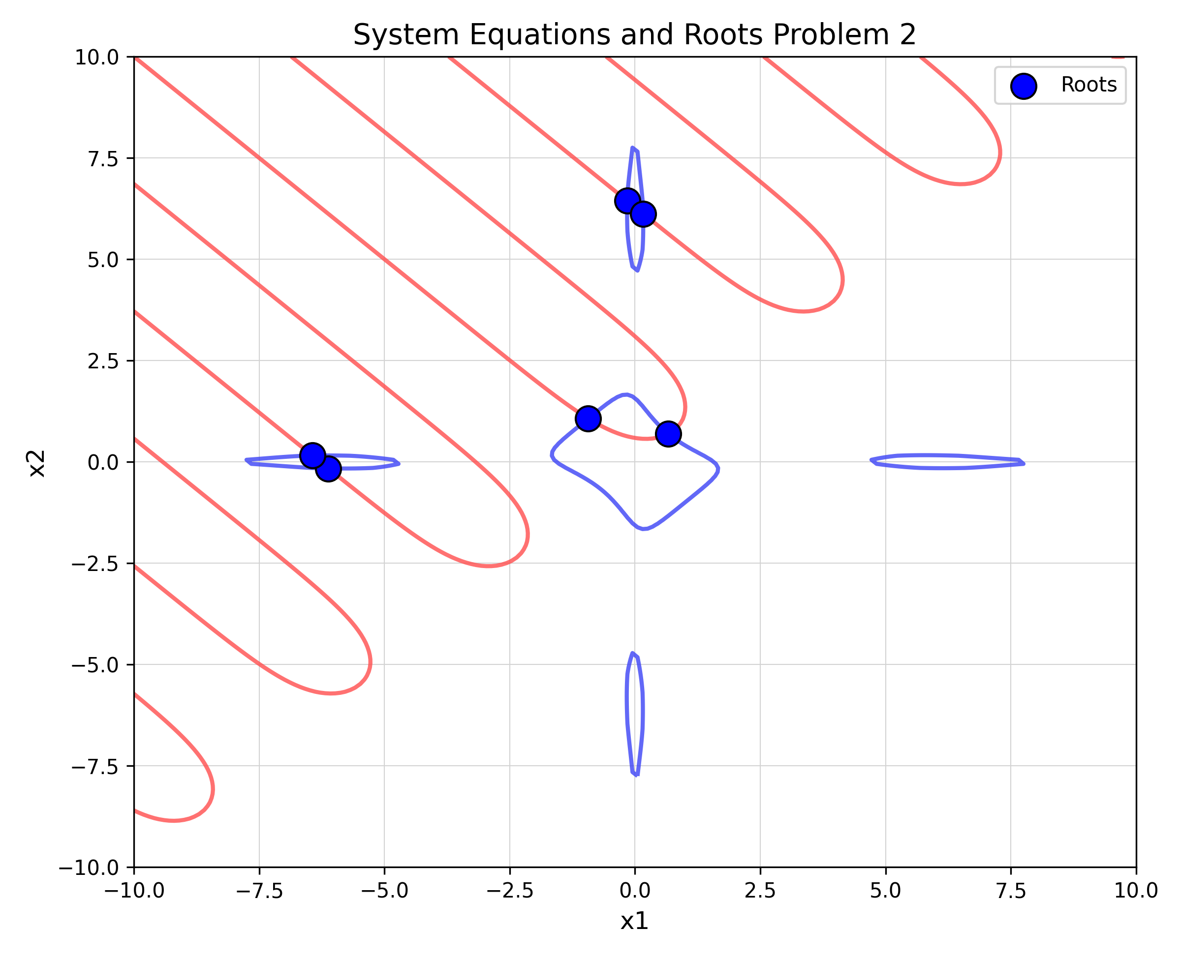
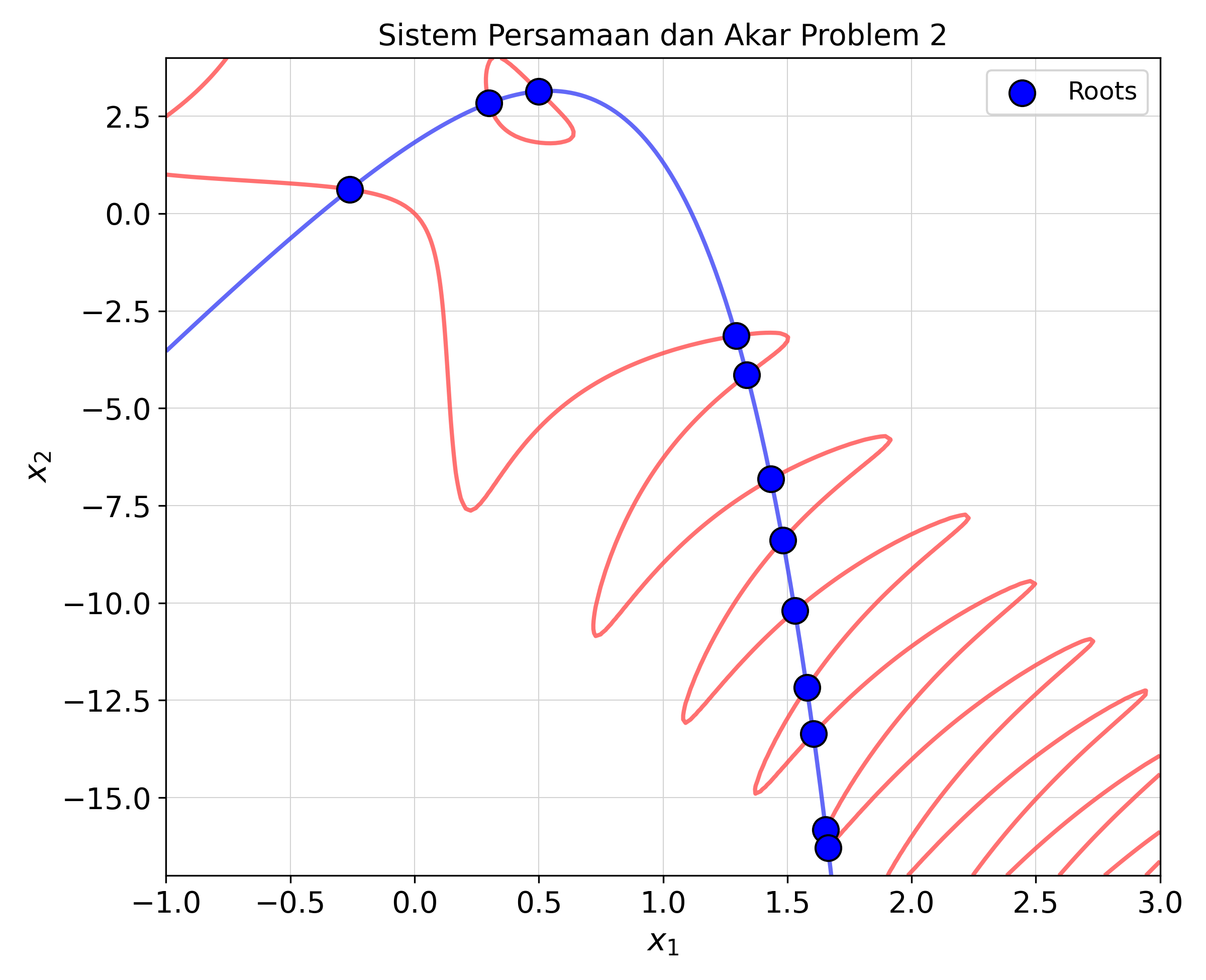
1. Visualizing SNE Systems & Discovered Roots

Run visualize_sne_results.py to solve an SNE benchmark problem and plot its zero-level equation contours overlaid with roots:

python examples/visualize_sne_results.py --problem 1 --save_dir ./plots --no_show

Output Plot:

python examples/visualize_sne_results.py --problem 2 --save_dir ./plots --no_show

Output Plot:

---

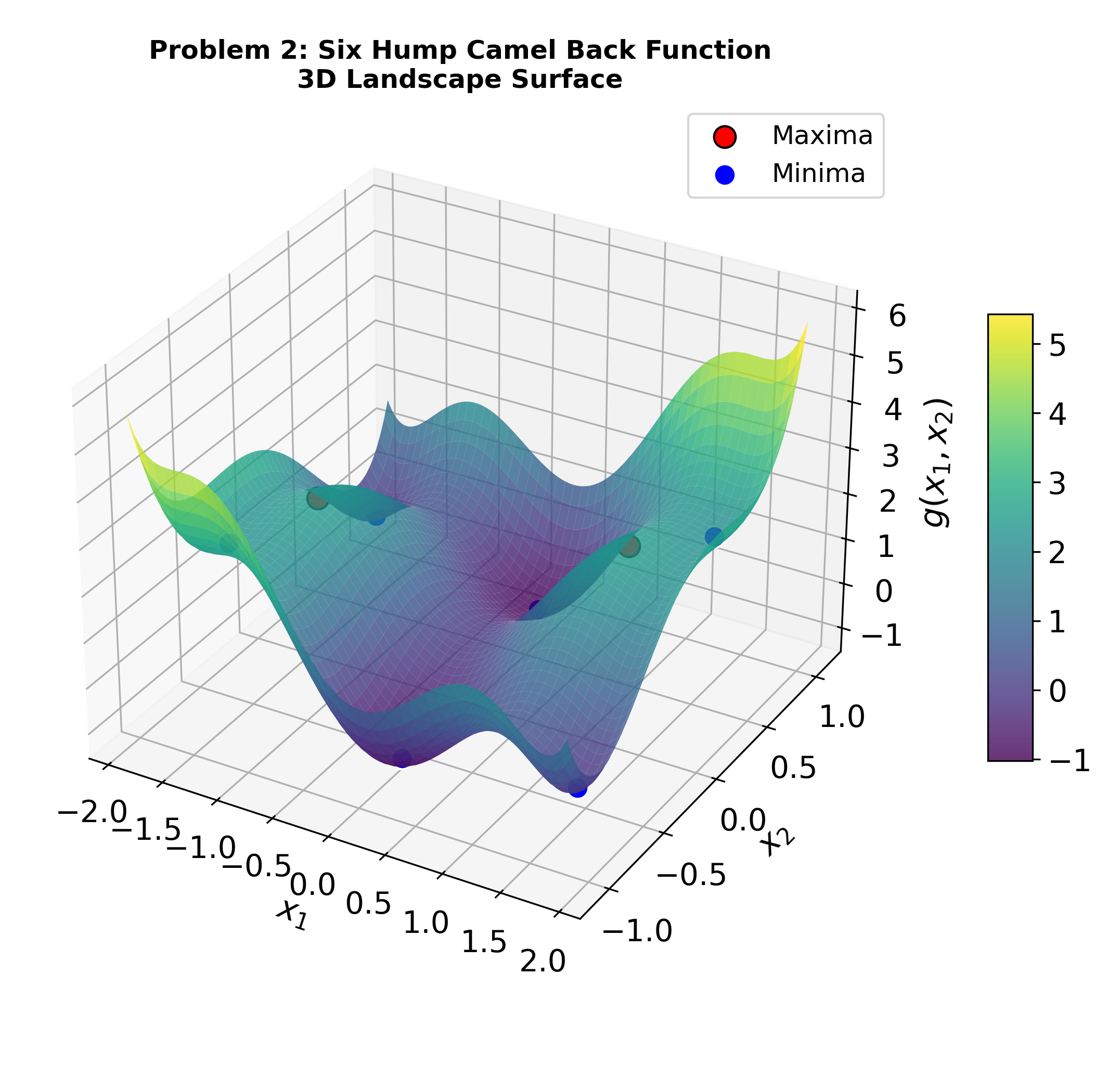
2. Visualizing Multimodal Landscapes & Optima

Run visualize_multimodal_results.py to inspect multimodal landscapes and overlay discovered maxima and minima:

python examples/visualize_multimodal_results.py --problem 2 --save_dir ./plots --no_show

Output Plot:

---

Command Line Arguments Reference

Argument	Type	Default	Description
--problem	str / int	1 (SNE) / 2 (Multimodal)	Problem key/ID from benchmark problem sets (benchmarks_sne or benchmarks_multimodal).
--save_dir	str	.	Directory path where output PNG images will be saved.
--no_show	flag	False	When set, saves figures directly to disk without displaying interactive pop-up windows.

---

Custom Problem Tutorial (Python API)

You can import pysne visualization functions into any custom Python workflow directly from pysne.visualization:

Example 1: Custom Multimodal Landscape

import numpy as np
from pysne.problems.base import MultimodalProblem
from pysne.visualization import plot_2d_multimodal_results

class MyCustomMultimodal(MultimodalProblem):
    @property
    def name(self):
        return "My Custom Landscape"

    def get_info(self):
        domain = [(-3.0, 3.0), (-3.0, 3.0)]
        return domain, {}

    def g_func(self, X):
        X = np.asarray(X)
        x1 = X[0] if X.ndim == 1 else X[:, 0]
        x2 = X[1] if X.ndim == 1 else X[:, 1]
        return np.sin(x1) * np.cos(x2)

# Instantiate problem and define discovered optima points
prob = MyCustomMultimodal()
maxima = np.array([[np.pi/2, 0.0]])
minima = np.array([[-np.pi/2, 0.0]])

# Render 3D Surface + 2D Contour plot
plot_2d_multimodal_results(prob, maxima, minima, save_path="custom_multimodal_results.png")

---

Example 2: Custom Non-linear System of Equations (SNE)

import numpy as np
from pysne.problems.base import SNEProblem
from pysne.visualization import plot_2d_sne_results

class MySNESystem(SNEProblem):
    @property
    def name(self):
        return "Circle & Line System"

    def get_equations(self):
        return [
            lambda x: x[0]**2 + x[1]**2 - 4,  # Circle of radius 2
            lambda x: x[0] - x[1]             # Line x1 = x2
        ]

    def get_info(self):
        domain = [(-3.0, 3.0), (-3.0, 3.0)]
        return domain, {}

# Instantiate problem and roots found by solver
prob = MySNESystem()
roots = np.array([
    [np.sqrt(2), np.sqrt(2)],
    [-np.sqrt(2), -np.sqrt(2)]
])

# Render zero-contour plot with overlaid roots
plot_2d_sne_results(prob, roots, save_path="custom_sne_results.png")

Python API Parameter Reference

All visualization functions (plot_1d_sne_results, plot_2d_sne_results, plot_2d_multimodal_results, etc.) accept the following optional output parameters:

Parameter	Type	Default	Description
save_path	str / None	None	Target filepath to save the output image (e.g., "output.png" or "./plots/my_plot.png"). If None, the image is not saved to disk automatically.
no_show	bool	False	Set to True to suppress plt.show() pop-up windows. Useful for automated scripts or headless environments.

Displaying in Jupyter Notebooks

When save_path=None in a Jupyter Notebook, plots automatically render inline. The visualization functions also return the Matplotlib Figure object, allowing further customization via fig.savefig("high_res.png", dpi=600).

---

View Source code for SNE Visualizer on GitHub View Source code for Multimodal Visualizer on GitHub